flowchart TB
  A["Same world<br/>20 cases, 80 non-cases, 100 total"]

  A --> B["Count<br/>20<br/>How many cases are there?"]
  A --> C["Probability<br/>20 out of 100 = 20%<br/>Cases out of everyone"]
  A --> D["Odds<br/>20 to 80 = 1:4<br/>Cases compared with non-cases"]
16 Odds vs Probability
16.1 Never Go in Against a Sicilian.
Westley sets two wine goblets on the table and lets Vizzini choose. One contains iocane powder. Vizzini does what he always does when uncertainty threatens his control: he turns reasoning into performance. A clever man, he says, would put the poison in front of his enemy. A cleverer man would expect that and reverse it. A still cleverer man would anticipate the reversal. With each turn, the logic sounds more refined. With each turn, Vizzini sounds more certain that the world has narrowed into something intelligence can solve.
What kills him is not the absence of logic but the acceptance of a false balance. Once he treats the choice as a clean two-world problem—poison here or poison there, one safe cup, one fatal cup—the rest is only elaboration. He keeps sharpening an argument built on the wrong comparison. Both goblets were poisoned. Westley survives because the structure of the scene was never the one Vizzini thought he was analyzing.
In statistics, the slippage is quieter but similar. The event itself can stay exactly the same while the comparison around it changes. Probability keeps the whole group in view: cases out of everyone. Odds compare cases with non-cases. Nothing about the underlying world has changed, but the denominator has, and that alone can make the same reality sound more ordinary, more dramatic, or more alarming than it did a line earlier.
One world, three different questions
To see that clearly, leave the goblets behind and move to a world whose structure is fully visible. Imagine a screening program with 100 people. Twenty truly have the condition. Eighty do not. Hold that world still.
Now ask three different questions of the same unchanged setting. If the question is simply how many cases there are, the answer is 20. That is the count. If the question is what share of the whole group has the condition, the answer is 20 out of 100, or 20%. That is the probability in this simple population view: cases out of everyone. If the question is how many cases there are compared with non-cases, the answer is 20 to 80, which simplifies to 1 to 4. That is the odds: cases compared with what remains.
Nothing about the underlying situation changed when the answers changed. The same 20 people are still cases. The same 80 are still non-cases. Only the denominator changed. Probability keeps the whole group in view, which is why it stays close to the everyday question most readers think they are asking: how common is this? Odds answer a more contrastive question: how many cases are there relative to the people without the outcome? Both descriptions are honest. They simply arrange the same reality differently, and arrangement is not a cosmetic matter. It shapes what the sentence seems to mean.
A whole-group denominator tends to preserve the question most readers think they are asking: how common is the outcome? A cases-versus-non-cases denominator invites a comparison instead. That shift is one reason odds are easy to mishear even when they are being reported correctly.
Keep the world fixed, change only the number of cases
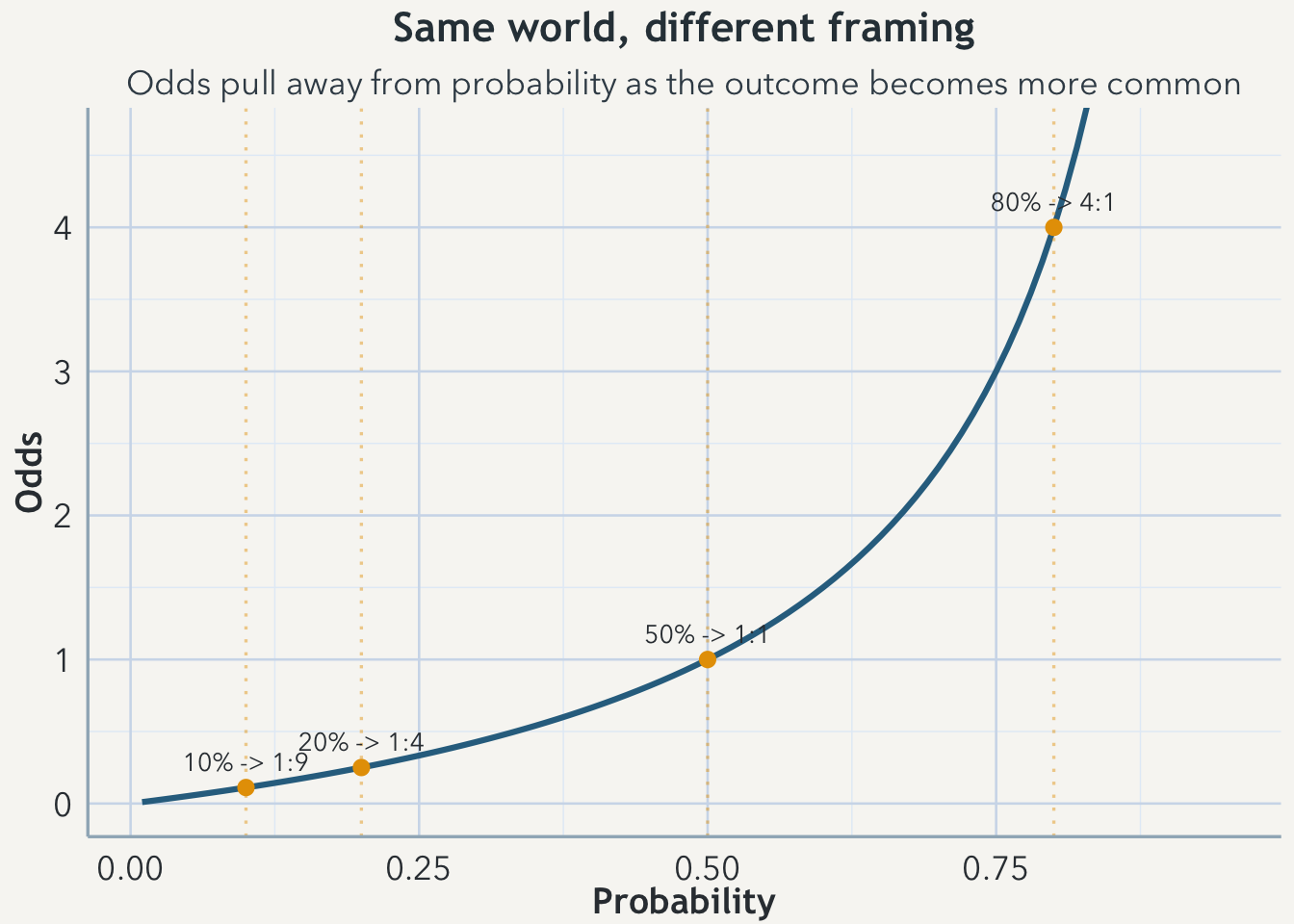
The distinction becomes easier to feel if the population stays fixed while the number of cases changes. Keep the group at 100 and vary only how many people have the condition. If 10 people are cases, the probability is 10% and the odds are 10 to 90, or about 1 to 9. If 20 people are cases, the probability is 20% and the odds are 1 to 4. If 50 people are cases, the probability is 50% and the odds are 1 to 1. If 80 people are cases, the probability is 80% and the odds are 4 to 1.
What matters is not only the arithmetic but the way the arithmetic feels. The world is changing steadily, yet odds begin to sound as though they are changing faster. That impression is not a mathematical mistake. It comes from the frame itself. Probability lives on the whole-population scale. Odds compare cases with whatever is left over. As the outcome becomes more common, the “what remains” part gets smaller, so odds pull away from probability more quickly and start to sound more extreme than the percentage alone.
Why an odds ratio is not the same thing as “double the probability”
This is the place where technically correct language often begins doing more rhetorical work than readers realize. If someone says the odds doubled, that may be exactly right on the odds scale. But many readers hear a different claim: that the underlying probability doubled in the same direct way. Sometimes the two are close. Often they are not.
A concrete example helps. Suppose one group starts with a 10% probability of the outcome. The odds are 1:9. If another group has twice those odds, the new odds are 2:9. Convert that back to probability and the result is not 20% but about 18%. Now start somewhere else. If the baseline probability is 50%, the odds are 1:1. If the odds double there, the new odds are 2:1, which translates back to a probability of about 67%, not 100%.
| Baseline probability | Baseline odds | Odds ratio | New odds | New probability | Change in probability |
|---|---|---|---|---|---|
| 10% | 1:9 | 2.0 | 2:9 | 18% | +8 percentage points |
| 50% | 1:1 | 2.0 | 2:1 | 67% | +17 percentage points |
The important point is not that odds ratios are suspect. It is that they live on a different scale. The same odds ratio can correspond to very different changes in probability depending on where the baseline starts. That is why odds-based model output can sound more dramatic than the practical change most readers are actually trying to imagine. Logistic regression often speaks in odds because that is the scale the model uses. Patients, practitioners, and policy readers usually do not think in odds. They think in chances, counts, and what those chances mean in a real group of people.
Why this matters in public health
Public-health claims rarely arrive in the tidy form used in a classroom. They come packaged as abstract conclusions, regression tables, dashboard annotations, press-release lines, and headlines written for speed. Sometimes the denominator is obvious. Sometimes it is buried. Sometimes the baseline risk is not given at all. Sometimes the dataset includes only the people who were tested, responded, showed up, or remained in follow-up, which means the world being described is already narrower than the sentence makes it sound.
The reading habit is plain even when the language around it is technical. How many cases are there? Out of how many total? Compared with what? And if the result is reported as odds, what would that claim look like again on the probability scale? Those questions do not simplify the analysis. They keep the analysis attached to the world it is supposed to describe.
Vizzini’s problem was not that he lacked a story about what was happening. It was that the story had accepted the wrong structure before the cleverness began. Statistical reading has the same vulnerability. Once the denominator changes, the picture changes with it. Probability and odds can both describe that picture honestly, but they do not ask the reader to imagine the same thing.
Takeaway
Probability answers a whole-group question: how common is the outcome in the population under discussion? Odds answer a comparative question: how many cases are there relative to non-cases? The important habit is to stop when you see odds, identify the denominator that is quietly structuring the claim, and translate the statement back into a world you can picture.